Question 707 continuously compounding rate, continuously compounding rate conversion
Convert a 10% effective annual rate ##(r_\text{eff annual})## into a continuously compounded annual rate ##(r_\text{cc annual})##. The equivalent continuously compounded annual rate is:
Question 711 continuously compounding rate, continuously compounding rate conversion
A continuously compounded semi-annual return of 5% ##(r_\text{cc 6mth})## is equivalent to a continuously compounded annual return ##(r_\text{cc annual})## of:
To compound up from semi-annual to annual, just multiply by 2 which is the number of 6 month periods in a year.
###\begin{aligned} r_\text{cc annual} &= r_\text{cc 6mth} \times 2 \\ &= 0.05 \times 2 \\ &= 0.1 \\ \end{aligned}###An effective semi-annual return of 5% ##(r_\text{eff 6mth})## is equivalent to an effective annual return ##(r_\text{eff annual})## of:
Converting effective rates to different time periods is requires powers to take compounding into effect. To compound up from semi-annual to annual, add one, raise to the power of 2, the number of semi-annual periods in a year, then subtract one.
###\begin{aligned} r_\text{eff annual} &= (1+r_\text{eff 6mth})^{2}-1 \\ &= (1+0.05)^{2}-1 \\ &= 0.1025 \\ \end{aligned}###Question 691 continuously compounding rate, effective rate, continuously compounding rate conversion, no explanation
A bank quotes an interest rate of 6% pa with quarterly compounding. Note that another way of stating this rate is that it is an annual percentage rate (APR) compounding discretely every 3 months.
Which of the following statements about this rate is NOT correct? All percentages are given to 6 decimal places. The equivalent:
No explanation provided.
If a variable, say X, is normally distributed with mean ##\mu## and variance ##\sigma^2## then mathematicians write ##X \sim \mathcal{N}(\mu, \sigma^2)##.
If a variable, say Y, is log-normally distributed and the underlying normal distribution has mean ##\mu## and variance ##\sigma^2## then mathematicians write ## Y \sim \mathbf{ln} \mathcal{N}(\mu, \sigma^2)##.
The below three graphs show probability density functions (PDF) of three different random variables Red, Green and Blue.
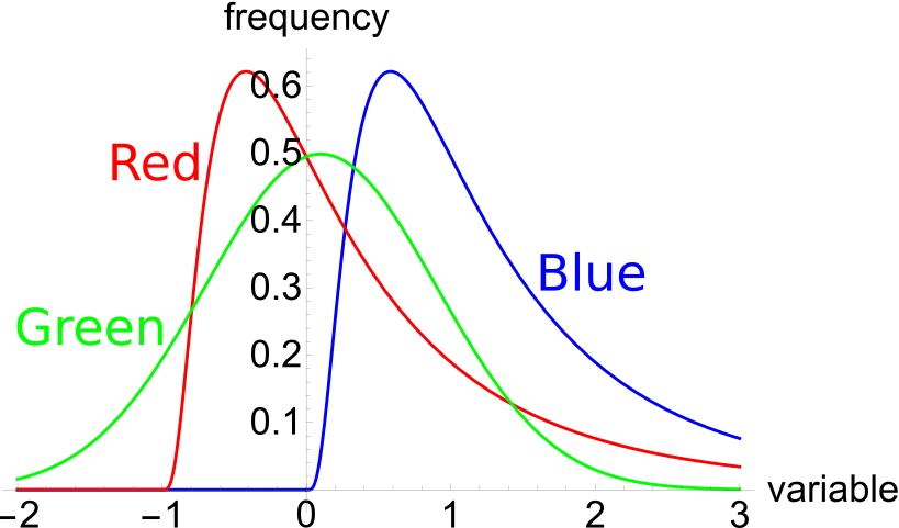
Select the most correct statement:
Variables Red and Blue are log-normally distributed since they are not symmetric, they're skewed. They have a fat right tail which stretches to positive infinity, but the left tail has a minimum point.
Variable Green has the symmetric bell-shape typical of a normal distribution which has left and right tails that continue to negative and positive infinity respectively.
The below three graphs show probability density functions (PDF) of three different random variables Red, Green and Blue. Let ##P_1## be the unknown price of a stock in one year. ##P_1## is a random variable. Let ##P_0 = 1##, so the share price now is $1. This one dollar is a constant, it is not a variable.
Which of the below statements is NOT correct? Financial practitioners commonly assume that the shape of the PDF represented in the colour:
The shape of the PDF represented in Red is commonly assumed to be the effective rate of return which is equal to the net discrete return. They are synonyms.
###r_\text{eff} = \text{NDR} = \text{GDR} - 1 = P_1/P_0-1 = (P_1-P_0)/P_0###The net discrete return equals the gross discrete return (Blue) minus one, which shifts the graph to the left by one unit. You can see that the Red PDF is the same as the Blue one, but shifted one unit to the left.
Note that the price and gross discrete return variables have the exact same PDF if the price now ##(P_0)## is one dollar, as stated in the assumptions. If the price is some other number, then the gross discrete return PDF will be a scaled version of stock price PDF since the gross discrete return is equal to the unknown future price divided by the known current price which is just a constant. For example, if the current stock price was $2 then the PDF of the price next year ##(P_1)## would look the same as the gross discrete return PDF but stretched along the x-axis to be twice as wide.
The mean of a normally distributed variable is always (asymptotically) equal to the median because the normal distribution is symmetric. Both the left and right tails are equal so outliers on each side tend to cancel each other out and do not affect either the median or mean (or mode). All three would be expected to be equal.
The mean of a log-normally distributed variable is always higher than the median because the median is the middle value (the 50th percentile) which is less influenced by outliers.
The mean is more heavily influenced by outliers, especially in the log-normal distribution where the mean is pulled higher by the very large returns in the fat right tail.
Question 719 mean and median returns, return distribution, arithmetic and geometric averages, continuously compounding rate
A stock has an arithmetic average continuously compounded return (AALGDR) of 10% pa, a standard deviation of continuously compounded returns (SDLGDR) of 80% pa and current stock price of $1. Assume that stock prices are log-normally distributed. The graph below summarises this information and provides some helpful formulas.
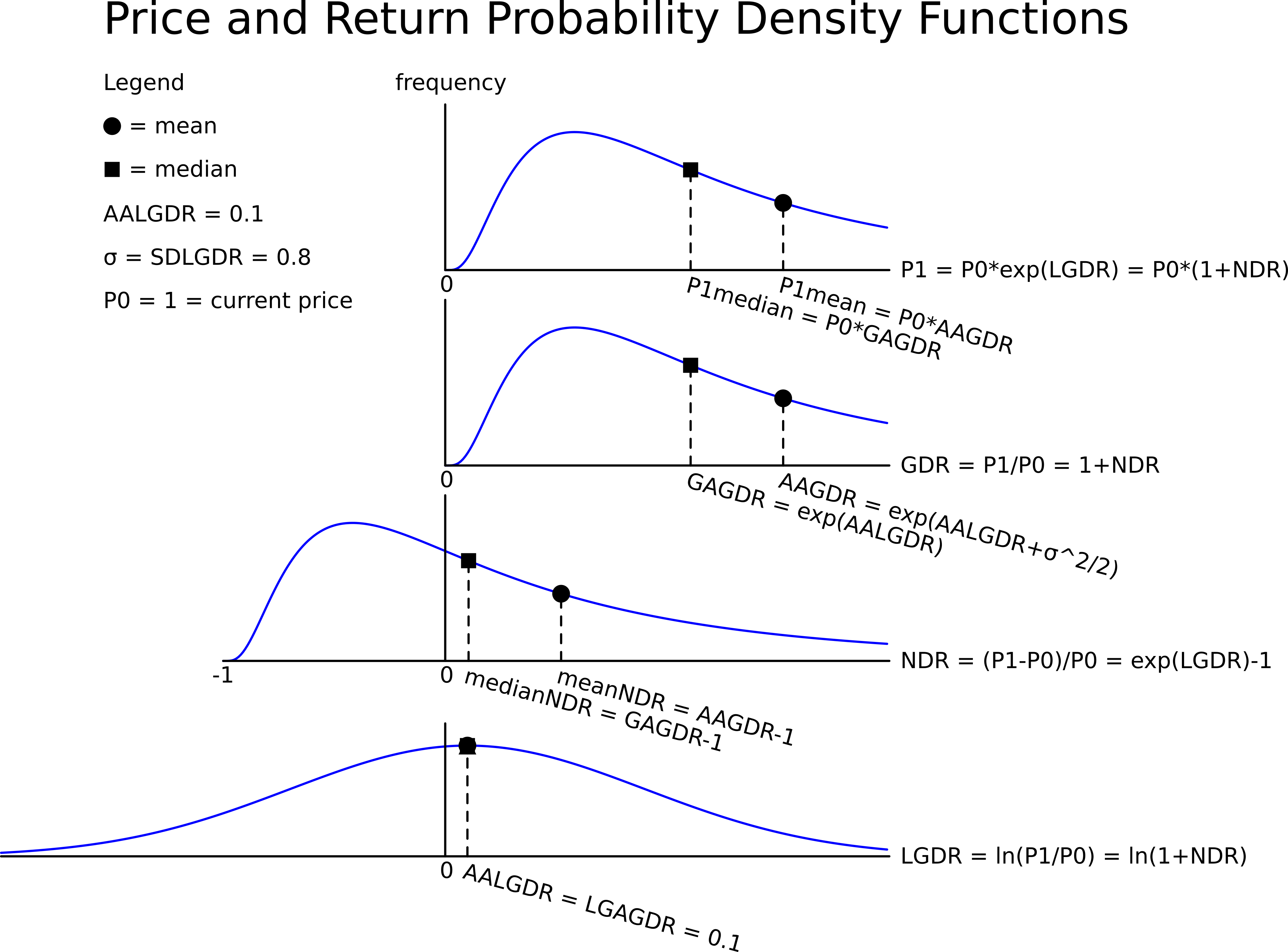
In one year, what do you expect the median and mean prices to be? The answer options are given in the same order.
The median price can be found by compounding up at the arithmetic average continuously compounded return ##(\text{AALGDR})##.
###\text{MedianP}_t = P_0.e^{\text{AALGDR}.t}### ###\begin{aligned} \text{MedianP}_{1} &= 1\times e^{0.1 \times 1} \\ &= 1.105170918 \\ \end{aligned}###The mean price can be found by compounding up at the arithmetic average continuously compounded return ##(\text{AALGDR})## plus half the variance ##(\text{SDLGDR}^2/2)##.
###\text{MeanP}_t = P_0.e^{(\text{AALGDR}+\text{SDLGDR}^2/2).t}### ###\begin{aligned} \text{MeanP}_{1} &= 1 \times e^{(0.1+0.8^2/2) \times 1} \\ &= 1.521961556 \\ \end{aligned}###
Question 720 mean and median returns, return distribution, arithmetic and geometric averages, continuously compounding rate
A stock has an arithmetic average continuously compounded return (AALGDR) of 10% pa, a standard deviation of continuously compounded returns (SDLGDR) of 80% pa and current stock price of $1. Assume that stock prices are log-normally distributed.
In 5 years, what do you expect the median and mean prices to be? The answer options are given in the same order.
The median price can be found by compounding up at the arithmetic average continuously compounded return ##(\text{AALGDR})##.
###\text{MedianP}_t = P_0.e^{\text{AALGDR}.t}### ###\begin{aligned} \text{MedianP}_{5} &= 1\times e^{0.1 \times 5} \\ &= 1.648721271 \\ \end{aligned}###The mean price can be found by compounding up at the arithmetic average continuously compounded return ##(\text{AALGDR})## plus half the variance ##(\text{SDLGDR}^2/2)##.
###\text{MeanP}_t = P_0.e^{(\text{AALGDR}+\text{SDLGDR}^2/2).t}### ###\begin{aligned} \text{MeanP}_{5} &= 1 \times e^{(0.1+0.8^2/2) \times 5} \\ &= 8.166169913 \\ \end{aligned}###Question 723 mean and median returns, return distribution, arithmetic and geometric averages, continuously compounding rate
Here is a table of stock prices and returns. Which of the statements below the table is NOT correct?
| Price and Return Population Statistics | ||||
| Time | Prices | LGDR | GDR | NDR |
| 0 | 100 | |||
| 1 | 99 | -0.010050 | 0.990000 | -0.010000 |
| 2 | 180.40 | 0.600057 | 1.822222 | 0.822222 |
| 3 | 112.73 | 0.470181 | 0.624889 | 0.375111 |
| Arithmetic average | 0.0399 | 1.1457 | 0.1457 | |
| Arithmetic standard deviation | 0.4384 | 0.5011 | 0.5011 | |
Statement b is false since it mixes the two average returns up.
###\exp \left( \text{GAGDR} \right) \neq \text{AALGDR}###The GAGDR equals the natural exponential of the arithmetic average of the logarithms of the gross discrete returns ##(\exp(\text{AALGDR})##.
###\begin{aligned} \text{GAGDR} &= \exp \left( \text{AALGDR} \right) \\ &= \exp \left( 0.0399 \right) \\ &= e^{0.0399} = 1.04075 \\ \end{aligned}###Statement a is true. The geometric average of the gross discrete returns (GAGDR) is equal to:
###\begin{aligned} \text{GAGDR} &= \left( \displaystyle\prod\limits_{t=1}^T{\left( \text{GDR}_t \right)} \right)^{1/T} \\ &= (0.990000 \times 1.822222 \times 0.624889)^{1/3} \\ &= 1.04075 = 104.075\% \\ \end{aligned}###Statement c is true. The geometric average gross discrete return is also equal to the last price divided by the first price raised to the power of the inverse number of time periods between them.
###\begin{aligned} \text{GAGDR} &= \left( P_T/P_0 \right)^{1/T} \\ &= (112.73/100)^{1/3} = 1.04075\\ \end{aligned}###Statement d is true. The logarithm of the geometric average of the gross discrete returns (LGAGDR) is equal to the arithmetic average of the logarithm of the gross discrete returns (AALGDR). This is always true, regardless of the distribution of returns.
###\text{LGAGDR} = \text{AALGDR}### Where: ###\text{LGAGDR} = \ln \left( \left( \displaystyle\prod\limits_{t=1}^T{\left( \text{GDR}_t \right)} \right)^{1/T} \right) ### ###\text{AALGDR} = \dfrac{ \displaystyle\sum\limits_{t=1}^T{\left( \text{LGDR}_t \right)} }{T} ###Let's check the equation using the table data:
###\ln(\text{GAGDR}) = \text{AALGDR}### ###\ln(1.04075) = 0.0399### ###0.0399 = 0.0399###Note that due to rounding in the GAGDR and AALGDR figures given in the table, the numbers aren't exactly equal after the 4th decimal place.
Statement e is true. The logarithm of the arithmetic average of the gross discrete returns (LAAGDR) is only asymptotically equal to the arithmetic average of the logarithm of the gross discrete returns (AALGDR) plus half the variance of the LGDR's. It's only true if the LGDR's are normally distributed and there are lots of observations.
###\text{LAAGDR} \approx \text{AALGDR} + \text{SDLGDR}^2/2###Note that ##\approx## means 'approximately equal to'. The equation will only be equal at the limit as the time period that the averages are measured over reaches infinity.
###\lim_{T \to \infty} (\text{AALGDR}) = \text{LGAGDR}###Let's check that the two sides of the equation are approximately equal using the table data:
###\text{LAAGDR} \approx \text{AALGDR} + \text{SDLGDR}^2/2### ###\ln(1.1457) \approx 0.0399 + 0.4384^2/2### ###0.136015804 = 0.13599728###So they are approximately equal, but the prices in the table were deliberately chosen to give this result. In actual stock price data with only 3 return observations such as here, the result would rarely hold.
Question 779 mean and median returns, return distribution, arithmetic and geometric averages, continuously compounding rate
Fred owns some BHP shares. He has calculated BHP’s monthly returns for each month in the past 30 years using this formula:
###r_\text{t monthly}=\ln \left( \dfrac{P_t}{P_{t-1}} \right)###He then took the arithmetic average and found it to be 0.8% per month using this formula:
###\bar{r}_\text{monthly}= \dfrac{ \displaystyle\sum\limits_{t=1}^T{\left( r_\text{t monthly} \right)} }{T} =0.008=0.8\% \text{ per month}###He also found the standard deviation of these monthly returns which was 15% per month:
###\sigma_\text{monthly} = \dfrac{ \displaystyle\sum\limits_{t=1}^T{\left( \left( r_\text{t monthly} - \bar{r}_\text{monthly} \right)^2 \right)} }{T} =0.15=15\%\text{ per month}###Assume that the past historical average return is the true population average of future expected returns and the stock's returns calculated above ##(r_\text{t monthly})## are normally distributed. Which of the below statements about Fred’s BHP shares is NOT correct?
The mean price in 10 years will be higher than the median price since the price must be log-normally distributed due to the continuously compounded return being normally distributed.
###\begin{aligned} \text{MeanPrice}_\text{10 years} &= \text{P}_\text{0} . e^{(AALGDR \mathbf{+} SDLGDR^2/2).t} \\ &= 20 \times e^{(0.008 + 0.15^2/2)×12×10} \\ &= 201.4884931 \\ \end{aligned}###The median price in 10 years is:
###\begin{aligned} \text{MedianPrice}_\text{10 years} &= \text{P}_\text{0} .e^{ \text{AALGDR}.t} \\ &= 20 \times e^{ 0.008 \times 12 \times 10} \\ &= 52.23392947 \\ \end{aligned}###The stock price is log-normally distributed so the mean will always be greater than the median.