Diversification is achieved by investing in a large amount of stocks. What type of risk is reduced by diversification?
Other names for diversifiable risk include:
- idiosyncratic risk
- firm-specific risk
- unique risk
- residual risk
- non-market risk
- non-systematic risk
Other names for systematic risk include:
- market risk
- undiversifiable risk
- beta risk
According to the CAPM, total risk is comprised of systematic and diversifiable risk. Mathematically, for some asset 'i':
###\text{total variance} = \text{systematic variance} + \text{idiosyncratic variance}### ###\begin{aligned} \sigma_\text{total, i}^2 &= \sigma_\text{systematic, i}^2 + \sigma_{\text{idiosyncratic, i}}^2 \\ &= \beta_i^2\sigma_\text{m}^2 + \sigma_{\epsilon\text{, i}}^2 \\ \end{aligned}\\###Idiosyncratic risk can be reduced by diversification but systematic risk can not.
According to the theory of the Capital Asset Pricing Model (CAPM), total risk can be broken into two components, systematic risk and idiosyncratic risk. Which of the following events would be considered a systematic, undiversifiable event according to the theory of the CAPM?
Systematic events affect a whole country and can't be avoided, such as an increase in a country's corporate tax rates. Diversifiable events affect only a specific company or industry or area, such as a firm's poor earnings announcement.
A fairly priced stock has an expected return equal to the market's. Treasury bonds yield 5% pa and the market portfolio's expected return is 10% pa. What is the stock's beta?
Since the stock is fairly priced, it must plot on the security market line (SML). It also has the same required return as the market portfolio. Therefore the stock must must have the same beta as the market, which is one.
A more mathematical answer can be shown using the CAPM's SML equation. Let the stock be 'i'.
###\mu_i = r_f + \beta_i(\mu_m - r_f)### ###0.1 = 0.05 + \beta_i(0.1 - 0.05)### ### \beta_i = 1###In case you're interested in why the market's beta is one, read on. The market's beta must be one because the covariance of the market portfolio's returns with itself is its variance of returns, and this divided by the same variance equals one.
Using the Greek symbols typically used in statistics:
###\begin{aligned} \beta_i &= \dfrac{\sigma_{i,M}}{\sigma_i.\sigma_M} \\ \beta_M &= \dfrac{\sigma_{M,M}}{\sigma_M.\sigma_M} \\ &= \dfrac{\sigma_{M}^2}{\sigma_M^2} \\ &= 1 \\ \end{aligned}###Using the statistical function names instead:
###\begin{aligned} \beta_i &= \dfrac{cov(r_i,r_M)}{std(r_i).std(r_M)} \\ \beta_M &= \dfrac{cov(r_M,r_M)}{std(r_M).std(r_M)} \\ &= \dfrac{var(r_M)}{var(r_M)} \\ &= 1 \\ \end{aligned}###The security market line (SML) shows the relationship between beta and expected return.
Buying investment projects that plot above the SML would lead to:
Investment assets that plot above the SML are:
- Expected to over-perform, having a positive abnormal return or 'alpha';
- Under-priced, the price is cheap;
- Positive NPV decisions when bought by buyers, and negative NPV decisions when sold by sellers.
Note that the SML relates beta (a measure of systematic risk) to expected return, so it only accounts for systematic risk and can not be used to gauge diversifiable risk or total risk.
Stock A has a beta of 0.5 and stock B has a beta of 1. Which statement is NOT correct?
All statements are true except the last phrase in answer (c). The market has a beta of one by definition, and so does stock B. Therefore they have the same level of systematic risk.
But total risk is comprised of systematic and diversifiable risk. Let a stock be represented by 'i'. When risk is measured using variance, then the following equation breaks any stock i's total variance into its systematic and idiosyncratic variances:
###\begin{aligned} \sigma_\text{i, total}^2 &= \beta_i^2.\sigma_m^2 + \sigma_\text{i, diversifiable}^2 \\ &= \sigma_\text{i, systematic}^2 + \sigma_\text{i, diversifiable}^2 \\ \end{aligned} ###
The market portfolio has no diversifiable variance since it is fully diversified. Stock B, on the other hand, is likely to have significant diversifiable variance since it is a single stock. Therefore stock B is likely to have higher total variance than the market portfolio since it has more diversifiable variance.
Which statement is the most correct?
According to the CAPM:
- beta is measured as:
###\begin{aligned} \beta_{i} &= \frac{\sigma_{i,m}}{\sigma_m^2} = \frac{cov(r_i, r_m)}{var(r_m)} \\ \end{aligned} ###
- total variance is the sum of systematic and idiosyncratic variances:
###\begin{aligned} \sigma_\text{i,total}^2 &= \beta_i^2.\sigma_m^2 + \sigma_\text{i,diversifiable}^2 \\ &= \sigma_\text{i,systematic}^2 + \sigma_\text{i,diversifiable}^2 \\ \end{aligned} ###
The risk free rate ##r_f## does not vary, it is a constant, therefore it has zero systematic and idiosyncratic variance and its beta is zero:
###\begin{aligned} \beta_{f} &= \frac{\sigma_{f,m}}{\sigma_m^2} = \frac{0}{\sigma_m^2} = 0 \\ \end{aligned} ###
The market portfolio is a portfolio of risky assets so it has a variance, but by definition its beta is one since the covariance of an asset with itself is equal to its variance:
###\begin{aligned} \beta_{m} &= \frac{\sigma_{m,m}}{\sigma_m^2} = \frac{\sigma_m^2}{\sigma_m^2} = 1 \\ \end{aligned} ###
The market portfolio has no idiosyncratic variance because it is fully diversified, and this makes sense since, using the total variance equation:
###\begin{aligned} \sigma_\text{i,total}^2 &= \beta_i^2.\sigma_\text{m,total}^2 + \sigma_\text{i,diversifiable}^2 \\ \sigma_\text{m,total}^2 &= \beta_m^2.\sigma_\text{m,total}^2 + \sigma_\text{m, diversifiable}^2 \\ &= 1^2.\sigma_\text{m,total}^2 + \sigma_\text{m,diversifiable}^2 \\ &= \sigma_\text{m,total}^2 + \sigma_\text{m,diversifiable}^2 \\ \sigma_\text{m,diversifiable}^2 &= \sigma_\text{m,total}^2 - \sigma_\text{m,total}^2 \\ &= 0 \\ \end{aligned} ###
Therefore the risk free rate has no risk at all so it has zero systematic and diversifiable (or idiosyncratic) risk, and the market portfolio has zero idiosyncratic risk.
A stock's correlation with the market portfolio increases while its total risk is unchanged. What will happen to the stock's expected return and systematic risk?
Let the stock be 'i' and the market portfolio be 'm', then:
###\begin{aligned} \beta_{i} &= \frac{cov(r_i, r_m)}{var(r_m)} &&= \frac{\sigma_{i,m}}{\sigma_m^2}\\ &= \frac{corr(r_i, r_m).std(r_i).std(r_m)}{var(r_m)} &&= \frac{\rho_{i,m}.\sigma_i.\sigma_m}{\sigma_m^2} \\ &= \frac{corr(r_i, r_m).std(r_i)}{std(r_m)} &&= \frac{\rho_{i,m}.\sigma_i}{\sigma_m} \\ \end{aligned} ###
So an increase in the correlation of returns between the stock and the market will increase the beta of the stock.
Using the CAPM's Security Market Line (SML) equation:
###\mu_i = r_f + \beta_i(\mu_m-r_f) ###An increase in the stock's beta (##\beta_i##) will increase the stock's expected return (##\mu_i##).
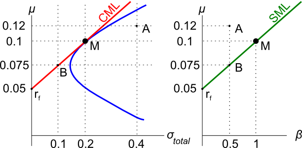
Assets A, B, M and ##r_f## are shown on the graphs above. Asset M is the market portfolio and ##r_f## is the risk free yield on government bonds. Which of the below statements is NOT correct?
The net present value (NPV) of buying asset A would be positive since it plots above the security market line (SML), it has a positive Jensen's alpha, because it is under-priced.
The net present value (NPV) of buying asset B would be zero since it plots on the security market line (SML), it has a zero Jensen's alpha, because it is fairly priced.
Assets A, B, M and ##r_f## are shown on the graphs above. Asset M is the market portfolio and ##r_f## is the risk free yield on government bonds. Assume that investors can borrow and lend at the risk free rate. Which of the below statements is NOT correct?
If risk-averse investors were forced to invest all of their wealth in a single risky asset A or B (not M since it's a portfolio) then they cannot diversify so total risk is important to them, not just systematic risk. Total risk is shown on the left graph's x-axis. Total variance equals systematic variance plus diversifiable variance:
###\text{TotalVariance} = \text{SystematicVariance} + \text{IdiosyncraticVariance}### ###\begin{aligned} \sigma_\text{total i}^2 &= \sigma_\text{systematic i}^2 + \sigma_{\text{idiosyncratic i}}^2 \\ &= \beta_i^2\sigma_\text{m}^2 + \sigma_{\epsilon\text{ i}}^2 \\ \end{aligned}\\###People who prefer low risk will choose asset B instead of A since ##\sigma_\text{B total} = 0.1## is less than ##\sigma_\text{B total}= 0.4##.
They're the sort of people who might carry an umbrella in their bag even when it's sunny, just in case it might rain. They suffer carrying it around but occasionally it helps them avoid getting drenched and sick. Or perhaps they purchase comprehensive car insurance. They're afraid of risk and are prepared to suffer low expected (average) returns to avoid large losses.
People who prefer high returns will choose asset A instead of B since ##\mu_A = 0.12## is greater than ##\mu_B = 0.075##.
They're the sort of people who may not purchase comprehensive car insurance because they're comfortable with the possibility of crashing their car and losing a large sum to replace it, if it means that they will have more money otherwise. They're comfortable with the possibility of suffering large losses if it means that on average they could gain more.
Choosing asset A or B is a personal choice, there's no correct answer. It depends on your return versus risk preferences. Of course in reality, you're not restricted to choose between A or B, you can choose a bit of both by making a portfolio which is the best idea.
A stock has a beta of 1.5. The market's expected total return is 10% pa and the risk free rate is 5% pa, both given as effective annual rates.
What do you think will be the stock's expected return over the next year, given as an effective annual rate?
A stock has a beta of 1.5. The market's expected total return is 10% pa and the risk free rate is 5% pa, both given as effective annual rates.
In the last 5 minutes, bad economic news was released showing a higher chance of recession. Over this time the share market fell by 1%. The risk free rate was unchanged.
What do you think was the stock's historical return over the last 5 minutes, given as an effective 5 minute rate?
Over the last 5 minutes, the return on the risk free rate would be close to zero ##(r_{f\text{ 5 min}} \approx 0)## since it's only 5% per year. The historical market return ##(r_{m\text{ 5 min}})## over the last 5 minutes was -1%. Note that in the CAPM equation below all returns are effective 5 minute historical returns. Substituting this into the CAPM equation: ###\begin{aligned} r_{i\text{ 5 min}} &= r_{f\text{ 5 min}} + \beta_i(r_{m\text{ 5 min}}-r_{f\text{ 5 min}}) \\ &= 0 + 1.5 \times (-0.01-0) \\ &= -0.015 \\ \end{aligned} ###
Discussion of why the 5 minute risk free rate is close to zero
To find the exact 5 minute risk free rate and show that it is truly close to zero, let's convert this 5% effective annual risk free rate into an effective 5 minute risk free rate. Assume that there are 365 days per year, 24 hours per day, 60 minutes per hour and therefore 12 (=60/5) five minute periods per hour.
###(1+r_{f\text{ 5 min}})^\text{number of 5 min periods in a year} = (1+r_{f\text{ annual}})^1### ###(1+r_{f\text{ 5 min}})^{365 \times 24 \times 60 / 5} = (1+r_{f\text{ annual}})### ###\begin{aligned} r_{f\text{ 5 min}} &= (1+r_{f\text{ annual}})^{1/(365 \times 24 \times 60 / 5)}-1 \\ &= (1+0.05)^{1/(365 \times 24 \times 60 / 5)}-1 \\ &= 0.000000464137895 \text{ pa} \\ &= 0.0000464137895 \text{% pa} \\ &\approx 0\text{% pa} \end{aligned}###A stock has a beta of 1.5. The market's expected total return is 10% pa and the risk free rate is 5% pa, both given as effective annual rates.
Over the last year, bad economic news was released showing a higher chance of recession. Over this time the share market fell by 1%. So ##r_{m} = (P_{0} - P_{-1})/P_{-1} = -0.01##, where the current time is zero and one year ago is time -1. The risk free rate was unchanged.
What do you think was the stock's historical return over the last year, given as an effective annual rate?
Over the last year, the historical effective return on the risk free rate was 5% ##(r_f = 0.05)##. The historical market return ##(r_m)## over the last year was -1% ##(r_m = -0.01)##. Note that in the CAPM equation below all returns are effective annual historical returns. Substituting this into the CAPM equation: ###\begin{aligned} r_i &= r_f + \beta_i(r_m-r_f) \\ &= 0.05 + 1.5 \times (-0.01-0.05) \\ &= -0.04 \\ \end{aligned} ###
A firm changes its capital structure by issuing a large amount of equity and using the funds to repay debt. Its assets are unchanged. Ignore interest tax shields.
According to the Capital Asset Pricing Model (CAPM), which statement is correct?
Beta (##\beta##) is a measure of systematic risk, along with variance (##\sigma^2##) and standard deviation (##\sigma##) .
Since the firm's assets (V) are funded by debt (D) and equity (E), the systematic risk of the firm's assets equals the weighted average beta of the debt and equity, so: ###\beta_V = \frac{D}{V}\beta_D + \frac{E}{V}\beta_E###
In this question, there is no change in the firm's assets. Therefore, all things remaining equal, there shouldn't be any change in the beta of the firm's assets (##\beta_V##).
Since the firm is issuing more equity (using a rights issue or private placement for example) and using the funds to repay debt (paying back the bond or loan-holders), the amount of equity will increase (↑ E) and the amount of debt will decrease (↓ D).
Equity holders have a residual claim on the firm's assets, which means that they get paid last if the firm goes bankrupt. So shareholders get paid after debt holders. Therefore the decrease in the amount of debt means that the equity holders are more likely to receive some payment if the firm goes bankrupt. It also means that there will be a smaller amount of interest payments that the firm must meet so there is a lower chance of going bankrupt. This means that equity must have less systematic risk, so it's beta will fall (↓##\beta_E##). This is the answer.
Also note that since there are less debt-holders, the smaller amount of debt also has less systematic risk (↓##\beta_D##). This may appear impossible since how can the beta on debt and equity fall, while the beta on assets remain constant? But this is possible since the beta on debt is always less than the beta on equity (##\beta_D < \beta_E##), and while both betas fall, there is a lower weight on debt (↓##\frac{D}{V}##), and a higher weight on equity (↑##\frac{E}{V}##), so the beta on assets stays the same.
To summarise: ###\overbrace{\beta_V}^{\cdot} = \overbrace{\frac{D}{V}}^{\downarrow} \overbrace{\beta_D}^{\downarrow} + \overbrace{\frac{E}{V}}^{\uparrow} \overbrace{\beta_E}^{\downarrow} ###
The CAPM can be used to find a business's expected opportunity cost of capital:
###r_i=r_f+β_i (r_m-r_f)###
What should be used as the risk free rate ##r_f##?
Strictly, cash flows in one month should be matched with required returns over the next one month, and cash flows in 10 years should be matched with required returns over the next ten years. This means that the required total return (same as the opportunity cost of capital), and the risk free rate and market portfolio rate used to calculate the required return, should always match the timing of the cash flows.
But in practice, since using multiple discount rates is too cumbersome, most analysts simply assume that required returns don't change significantly over time. Analysts tend to use the longest term government bond yield available. This makes some sense since most businesses are a 'going concern', meaning that they are supposed to continue forever. Therefore the cash flows are expected to go forever so the required total return should be measured over a long period.
Note that the current long term government bond yield is more useful than the historical government bond yield since we're trying to find the present value of future cash flows, not past cash flows.
The choice of which government bond yield to use as the risk free rate is a hotly debated topic, as is the existence of a truly risk-free rate at all.
A firm's WACC before tax would decrease due to:
The WACC before tax, also known as the opportunity cost of capital or the required return on assets (##r_{VL}##), will decrease when the firm's systematic risk decreases. This is because the WACC before tax takes the time value of money and the systematic risk into account. This is apparent when you consider the two different ways to calculate the WACC before tax.
There is the familiar formula which is the weighted average cost of the equity and debt used to finance the firm's assets:
###r_\text{WACC before tax} = r_{VL} = {r_D.\frac{D}{V_L} + r_{EL}.\frac{E_L}{V_L}}###Since ##V=D+E##, this should be equal to the required return on the firm's assets using the CAPM with the firm's asset beta:
###r_\text{WACC before tax} = r_{VL} = {r_f} + \beta_{VL}(r_m - r_f)###This CAPM version of the WACC before tax equation breaks the required return into the time value of money (##r_f##) and the systematic risk premium (##\beta_{VL}(r_m - r_f)##).
Clearly, the lower the levered asset beta (##\beta_{VL}##), the lower the WACC before tax.
Note that the WACC before tax is not affected by tax shields, unlike the WACC after tax. Therefore an increase in debt and tax shields (answer c) or a decrease (answer d) will have no effect. But the WACC after tax will decrease and increase respectively.
Which of the following statements about the weighted average cost of capital (WACC) is NOT correct?
The WACC after-tax includes the benefit of the tax shield by reducing the cost of debt. Answer (e) is incorrect since it is simply the before-tax WACC without any adjustment for the benefit of the tax shield. Read on for a more detailed look at each type of WACC equation.
WACC before taxThe WACC before tax, also known as the opportunity cost of capital or the required return on assets (##r_{VL}##), takes the time value of money and the systematic risk into account. This is apparent when you consider the two different ways to calculate the WACC before tax.
There is the familiar formula which is the weighted average cost of the equity and debt used to finance the firm's assets:
###r_\text{WACC before tax} = r_D.\frac{D}{V_L} + r_{EL}.\frac{E_L}{V_L}###Since ##V=D+E##, this should be equal to the required return on the firm's assets using the CAPM with the firm's asset beta:
###r_\text{WACC before tax} = r_{VL} = {r_f} + \beta_{VL}.(r_m - r_f)###This CAPM version of the WACC before tax equation breaks the required return into the time value of money (##r_f##) and the systematic risk premium (##\beta_{VL}.(r_m - r_f)##).
WACC after-taxThe WACC after-tax is just the same as the WACC before-tax, but it also includes the benefit of the tax shield. The WACC after-tax can also be represented by two formulas, the first and last written here:
###\begin{aligned} r_\text{WACC after tax} &= r_D.(1-t_c).\frac{D}{V_L} + r_{EL}.\frac{E_L}{V_L} \\ &= {r_D.\frac{D}{V_L} + r_{EL}.\frac{E_L}{V_L}} - r_D.t_c.\frac{D}{V_L}\\ &= r_\text{WACC before tax} - r_D.t_c.\frac{D}{V_L}\\ &= {r_f} + \beta_{VL}.(r_m - r_f) - r_D.t_c.\frac{D}{V_L}\\ \end{aligned}###
Question 418 capital budgeting, NPV, interest tax shield, WACC, CFFA, CAPM
| Project Data | ||
| Project life | 1 year | |
| Initial investment in equipment | $8m | |
| Depreciation of equipment per year | $8m | |
| Expected sale price of equipment at end of project | 0 | |
| Unit sales per year | 4m | |
| Sale price per unit | $10 | |
| Variable cost per unit | $5 | |
| Fixed costs per year, paid at the end of each year | $2m | |
| Interest expense in first year (at t=1) | $0.562m | |
| Corporate tax rate | 30% | |
| Government treasury bond yield | 5% | |
| Bank loan debt yield | 9% | |
| Market portfolio return | 10% | |
| Covariance of levered equity returns with market | 0.32 | |
| Variance of market portfolio returns | 0.16 | |
| Firm's and project's debt-to-equity ratio | 50% | |
Notes
- Due to the project, current assets will increase by $6m now (t=0) and fall by $6m at the end (t=1). Current liabilities will not be affected.
Assumptions
- The debt-to-equity ratio will be kept constant throughout the life of the project. The amount of interest expense at the end of each period has been correctly calculated to maintain this constant debt-to-equity ratio.
- Millions are represented by 'm'.
- All cash flows occur at the start or end of the year as appropriate, not in the middle or throughout the year.
- All rates and cash flows are real. The inflation rate is 2% pa. All rates are given as effective annual rates.
- The project is undertaken by a firm, not an individual.
What is the net present value (NPV) of the project?
Because interest expense has been correctly calculated so that a constant debt-to-equity ratio is maintained, there are a number of ways to do this question.
Textbook method or interest tax shield in the discount rate method
By ignoring interest expense ##(IntExp=0)## and finding the firm's free cash flow excluding interest tax shields ##(FFCF_\text{xITS})##, and then discounting by the weighted average cost of capital after tax ##(WACC_\text{after tax})##, the value of the firm including interest tax shields can be found.
To find the firm's free cash flows excluding the benefit of interest tax shields at time one:
###\begin{aligned} FFCF_\text{xITS, 0} &= NI_0 + Depr - CapEx - \Delta NWC + IntExp \\ &= 0 + 0 - 8m -6m + 0 \\ &= - 14m \\ \end{aligned}###The CapEx at time one is nothing since the equipment was worthless at the end of its life and its book value was also zero:
###\begin{aligned} CapEx_1 &= -\text{CapitalSalesAfterTax}_1 \\ &= -(P_\text{sale, 1} - \text{CapitalGainsTax}_1) \\ &= -(P_\text{sale, 1} - (P_\text{sale, 1} - P_\text{book, 1}).t_c) \\ &= -(P_\text{sale, 1} - (P_\text{sale, 1} - (P_\text{buy, 0} - Depr_1)).t_c) \\ &= -(0 - (0 - (8m - 8m)) \times 0.3) \\ &= 0 \\ \end{aligned}### ###\begin{aligned} NI_\text{xITS, 1 and 2} &= (Q.(P-VC) - FC - Depr - IntExp).(1-t_c) \\ &= (4m \times (10-5) - 2m - 8m - 0).(1-0.3) \\ & = 7m \\ \end{aligned}### ###\begin{aligned} FFCF_\text{xITS, 1} &= NI_\text{xITS, 1} + Depr - CapEx - \Delta NWC + IntExp \\ &= 7m + 8m - 0 - (-6m) + 0 \\ &= 21m \\ \end{aligned}###Now to find the WACC after tax. First convert the debt-to-equity ratio into a debt-to-assets ratio:
###\dfrac{D}{E} = \frac{0.5}{1}###So D could be 0.5 and E could be 1. Then:
###\dfrac{D}{V} = \dfrac{D}{D+E} = \dfrac{0.5}{0.5+1} = \dfrac{1}{3}###Now find the levered cost of equity using the CAPM. First we need the beta of levered equity:
###\begin{aligned} \beta_E &=\dfrac{cov(r_E, r_M)}{var(r_M)} \\ &=\dfrac{0.32}{0.16} \\ &= 2 \\ \end{aligned}### ###\begin{aligned} r_E &= r_f + \beta_E.(r_m-r_f) \\ &= 0.05 + 2 \times(0.1-0.05) \\ &= 0.15 \\ \end{aligned}###To find the WACC after tax:
###\begin{aligned} r_\text{WACC after tax} &= \dfrac{D}{V}.r_D.(1-t_c) + \dfrac{E}{V}.r_E \\ &= \dfrac{1}{3} \times 0.09 \times (1-0.3) + \dfrac{2}{3} \times 0.15 \\ &= 0.121 \\ \end{aligned}###Finally, find the value of the levered firm's assets with interest tax shields.
###\begin{aligned} V_\text{wITS, 0} &= FFCF_\text{xITS, 0} + \dfrac{FFCF_\text{xITS, 1}}{(1+r_\text{WACC after tax})^1} \\ &= -14 + \dfrac{21m}{(1+0.121)^1} \\ &= 4.733273863m \\ \end{aligned}###