Question 708 continuously compounding rate, continuously compounding rate conversion
Convert a 10% continuously compounded annual rate ##(r_\text{cc annual})## into an effective annual rate ##(r_\text{eff annual})##. The equivalent effective annual rate is:
Which of the following interest rate quotes is NOT equivalent to a 10% effective annual rate of return? Assume that each year has 12 months, each month has 30 days, each day has 24 hours, each hour has 60 minutes and each minute has 60 seconds. APR stands for Annualised Percentage Rate.
Since the assumptions state that there are 30 days per month and therefore 360 days per year, then the annualised percentage rate compounding per day should be:
###\begin{aligned} r_\text{APR comp daily} &= r_\text{eff daily} \times 360 \\ &= ((1 + r_\text{eff annual})^{1/360}-1) \times 360 \\ &= ((1 + 0.1)^{1/360}-1) \times 360 \\ &= 0.00026478555 \times 360 \\ &= 0.095322798 \\ \end{aligned}###Commentary
Notice that the APR's get smaller as the compounding period becomes shorter. The continuously compounded return is the limit when the compounding period is infinitely small. The APR compounding per second is nearly equal to the continuously compounded rate.
| Different Return Quotations Equivalent to an Effective Annual Rate of 10% | ||||
| Quote type | Return (%pa) | Symbol | Formula | Spreadsheet formula |
| Effective annual rate | 10 | ##r_\text{eff annual}## | ##=r_\text{eff annual}## | =0.1 |
| APR compounding per annum | 10 | ##r_\text{apr comp annually}## | ##=r_\text{eff annual}## | =0.1 |
| APR compounding semi-annually | 9.761769634 | ##r_\text{apr comp 6mth}## | ##=2 \times ((1+r_\text{eff annual})^{1/2}-1)## | =2 * ((1+0.1)^(1/2)-1) |
| APR compounding quarterly | 9.645475634 | ##r_\text{apr comp quarterly}## | ##=4 \times ((1+r_\text{eff annual})^{1/4}-1)## | =4 * ((1+0.1)^(1/4)-1) |
| APR compounding monthly | 9.568968515 | ##r_\text{apr comp monthly}## | ##=12 \times ((1+r_\text{eff annual})^{1/12}-1)## | =12 * ((1+0.1)^(1/12)-1) |
| APR compounding daily | 9.532279763 | ##r_\text{apr comp daily}## | ##=360\times ((1+r_\text{eff annual})^{1/360}-1)## | =360 * ((1+0.1)^(1/360)-1) |
| APR compounding hourly | 9.531070550 | ##r_\text{apr comp hourly}## | ##=360 \times 24 \times ((1+r_\text{eff annual})^{1/(360 \times 24)}-1)## | =360*24 * ((1+0.1)^(1/(360*24))-1) |
| APR compounding per minute | 9.531018861 | ##r_\text{apr comp per minute}## | ##=360 \times 24 \times 60 \times ((1+r_\text{eff annual})^{1/(360 \times 24 \times 60)}-1)## | =360*24*60 * ((1+0.1)^(1/(360*24*60))-1) |
| APR compounding per second | 9.531018227 | ##r_\text{apr comp per second}## | ##=360 \times 24 \times 60 \times 60 \times ((1+r_\text{eff annual})^{1/(360 \times 24 \times 60 \times 60)}-1)## | =360*24*60*60 * ((1+0.1)^(1/(360*24*60*60))-1) |
| Continuously compounded annual rate | 9.531017980 | ##r_\text{cc annual}## | ##=\ln(1+r_\text{eff annual}) = log_e(1+r_\text{eff annual})## | =ln(1+0.1) |
Question 710 continuously compounding rate, continuously compounding rate conversion
A continuously compounded monthly return of 1% ##(r_\text{cc monthly})## is equivalent to a continuously compounded annual return ##(r_\text{cc annual})## of:
Converting continuously compounding rates to different time periods is surprisingly easy. To compound up from monthly to annual, just multiply by the number of months in a year.
###\begin{aligned} r_\text{cc annual} &= r_\text{cc monthly} \times 12 \\ &= 0.01 \times 12 \\ &= 0.12 \\ \end{aligned}###An effective monthly return of 1% ##(r_\text{eff monthly})## is equivalent to an effective annual return ##(r_\text{eff annual})## of:
Converting effective rates to different time periods requires powers to take compounding into account. To compound up from monthly to annual, add one, raise to the power of the number of months in a year, then subtract one.
###\begin{aligned} r_\text{eff annual} &= (1+r_\text{eff monthly})^{12}-1 \\ &= (1+0.01)^{12}-1 \\ &= 0.12682503 \\ \end{aligned}###Which of the following quantities is commonly assumed to be normally distributed?
No explanation provided.
The below three graphs show probability density functions (PDF) of three different random variables Red, Green and Blue.
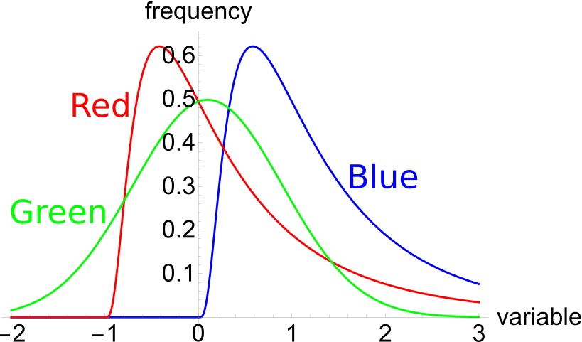
Which of the below statements is NOT correct?
The variable Green is always between ##-\infty < Green < \infty## if it is normally distributed, there is no minimum or maximum value. This is because a normal distribution has left and right tails that stretch to negative and positive infinity respectively.
The mean of a log-normally distributed variable is always higher than the median because the median is the middle value (the 50th percentile) which is less influenced by outliers.
The mean is more heavily influenced by outliers, especially in the log-normal distribution where the mean is pulled higher by the very large returns in the far right tail.
The symbol ##\text{GDR}_{0\rightarrow 1}## represents a stock's gross discrete return per annum over the first year. ##\text{GDR}_{0\rightarrow 1} = P_1/P_0##. The subscript indicates the time period that the return is mentioned over. So for example, ##\text{AAGDR}_{1 \rightarrow 3}## is the arithmetic average GDR measured over the two year period from years 1 to 3, but it is expressed as a per annum rate.
Which of the below statements about the arithmetic and geometric average GDR is NOT correct?
Statement b is false. The geometric average return is the product of the returns raised to the power of 1 on the number of returns:
###\text{GAGDR}_{0\rightarrow T} = \left( \text{GDR}_{0 \rightarrow 1} . \text{GDR}_{1\rightarrow 2} ... \text{GDR}_{T-1 \rightarrow T} \right)^{\mathbf{1/T}}###Statement e is true. The arithmetic and geometric averages of returns will be equal if the variance of the stock's returns is zero. But this would be very unusual because the stock return would then be constant and therefore risk free.
Question 811 log-normal distribution, mean and median returns, return distribution, arithmetic and geometric averages
Which of the following statements about probability distributions is NOT correct?
A stocks’ future annual net discrete returns ##(P_t/P_0-1)## must be log-normally distributed when future stock prices ##(P_t)## are also log-normally distributed. This is because net discrete returns are 'linear transformations' of stock prices. The shape of the net discrete return's distribution (given by its probability density function or PDF) is the same as the future stock price's log-normal distribution, but it's squashed flatter when it's divided by the original price ##(P_t/\color{red}{P_0}-1)##, and shifted to the left by one unit due to the minus one ##(P_t/P_0\color{red}{-1})##.
Question 721 mean and median returns, return distribution, arithmetic and geometric averages, continuously compounding rate
Fred owns some Commonwealth Bank (CBA) shares. He has calculated CBA’s monthly returns for each month in the past 20 years using this formula:
###r_\text{t monthly}=\ln \left( \dfrac{P_t}{P_{t-1}} \right)###He then took the arithmetic average and found it to be 1% per month using this formula:
###\bar{r}_\text{monthly}= \dfrac{ \displaystyle\sum\limits_{t=1}^T{\left( r_\text{t monthly} \right)} }{T} =0.01=1\% \text{ per month}###He also found the standard deviation of these monthly returns which was 5% per month:
###\sigma_\text{monthly} = \dfrac{ \displaystyle\sum\limits_{t=1}^T{\left( \left( r_\text{t monthly} - \bar{r}_\text{monthly} \right)^2 \right)} }{T} =0.05=5\%\text{ per month}###Which of the below statements about Fred’s CBA shares is NOT correct? Assume that the past historical average return is the true population average of future expected returns.
Over the next 10 years the expected mean gross discrete 10 year return is:
###\text{MeanGDR} = \text{AAGDR} = e^{(AALGDR + SDLGDR^2/2).t} = e^{(0.01 + 0.05^2/2)×12×10} = 3.857425531###The expected median gross discrete 10 year return is:
###\text{MedianGDR} = \text{GAGDR} = e^{AALGDR.t} = e^{0.01×12×10}=3.320116923###Note that the gross discrete return is log-normally distributed so the mean will always be greater than the median.
Question 722 mean and median returns, return distribution, arithmetic and geometric averages, continuously compounding rate
Here is a table of stock prices and returns. Which of the statements below the table is NOT correct?
| Price and Return Population Statistics | ||||
| Time | Prices | LGDR | GDR | NDR |
| 0 | 100 | |||
| 1 | 50 | -0.6931 | 0.5 | -0.5 |
| 2 | 100 | 0.6931 | 2 | 1 |
| Arithmetic average | 0 | 1.25 | 0.25 | |
| Arithmetic standard deviation | 0.9802 | 1.0607 | 1.0607 | |
Statement e is false and it can be verified using the actual data in the table, which is done below. The logarithm of the arithmetic average of the gross discrete returns (LAAGDR) is only asymptotically equal to the arithmetic average of the logarithms of the gross discrete returns (AALGDR) plus half the variance of the LGDR's. It's only true if the LGDR's are normally distributed and there are lots of observations.
###\text{LAAGDR} \approx \text{AALGDR} + \text{SDLGDR}^2/2###Note that ##\approx## means 'approximately equal to'. The equation will only be equal at the limit as the time period that the averages are measured over reaches infinity.
###\lim_{T \to \infty} (LAAGDR) = \lim_{T \to \infty} (\text{AALGDR} + \text{SDLGDR}^2/2)###Let's check that the two sides of the equation are approximately equal, but not exactly equal, using the table data:
###\text{LAAGDR} \approx \text{AALGDR} + \text{SDLGDR}^2/2### ###\ln(1.25) \approx 0 + 0.98019142^2/2### ###0.223143551 \approx 0.48038761###The figures are quite different, but if more time periods were added, then these values would converge to be approximately equal. One reason why the figures are different is because the two gross discrete return data points are not log-normally distributed. Remember that the log-normal distribution is supposed to be skewed but with only two return observations it's impossible to create skew.
Statement d is true. The logarithm of the geometric average of the gross discrete returns (LGAGDR) is equal to the arithmetic average of the logarithms of the gross discrete returns (AALGDR). This is always true, regardless of the distribution of returns.
###\text{LGAGDR} = \text{AALGDR}### Where: ###\text{LGAGDR} = \ln \left( \left( \displaystyle\prod\limits_{t=1}^T{\left( \text{GDR}_t \right)} \right)^{1/T} \right) ### ###\text{AALGDR} = \dfrac{ \displaystyle\sum\limits_{t=1}^T{\left( \text{LGDR}_t \right)} }{T} ###Let's check the equation using the table data:
###\ln(\text{GAGDR}) = \text{AALGDR}### ###\ln(1) = 0### ###0 = 0###Statement a is true. The geometric average of the gross discrete returns (GAGDR) is equal to:
###\text{GAGDR} = \left( \displaystyle\prod\limits_{t=1}^T{\left( \text{GDR}_t \right)} \right)^{1/T} = (0.5 \times 2)^{1/2} = 1 = 100\%###Interestingly, another way to calculate the GAGDR is to find the natural exponent of the arithmetic average of the logarithms of the gross discrete returns (AALGDR).
This means that statement b is also true:
###\text{GAGDR} = \exp \left( \text{AALGDR} \right) = \exp \left( 0 \right) = e^0 = 1###Statement c is true. The geometric average gross discrete return is also equal to the last price divided by the first price raised to the power of the inverse number of time periods between them.
###\text{GAGDR} = \left( P_T/P_0 \right)^{1/T} = (100/100)^{1/2} = 1 = 100\%###